Distributions

A distribution produces a random value each time it is sampled, so a model can reflect real variation instead of a single fixed number. Reach for one anywhere a value naturally varies: a processing time that is sometimes fast and sometimes slow, a batch size, or the gap between arrivals.

ProcessModel draws a fresh value every time the expression runs, from a repeatable random stream so a run can be reproduced exactly. A distribution can go in any numeric field: processing time, move time, arrival interval, quantity, or an attribute.

Two things that apply across all of them:

• A time can never be negative, so distributions that could return a negative number (such as Normal) have those draws clamped to 0.
• Most distributions have both a short alias and a long name; N(10,2) and Normal(10,2) are the same.

Common distributions

Each has its own page with the shape, the parameters, and when to reach for it:

• Triangular: T(min, mode, max), the everyday choice from three estimates.
• Uniform: U(min, max), every value in a range equally likely.
• Normal: N(mean, sd), values clustered around an average.
• Exponential: E(mean), the gap between random arrivals.
• Lognormal: Lognormal(mu, sigma), right-skewed task times.
• Beta: Beta(min, max, p, q), a flexible shape on a fixed range.
• Gamma: Gamma(shape, rate), the time for several steps.
• Weibull: Weibull(shape, scale), time to failure.
• Erlang: Erlang(stages, rate), a sum of exponential stages.
• Poisson: Poisson(mean), a count of events in a period.
• Binomial: Binomial(trials, p), successes out of a number of tries.
• Geometric: Geometric(p), tries until the first success.
• Negative Binomial: NegBinomial(successes, p), tries to reach several successes.
• Rayleigh: Rayleigh(scale), a skewed positive value from one parameter.

Discrete and data-driven

• Discrete: D2 to D5, pick from a few set values by percentage.
• User-Defined: UD('name'), build a distribution from your own data or value and percent pairs.

More distributions

ProcessModel also supports these less common distributions, entered the same way (the Expression Builder lists them all): ChiSquared(df), DiscreteUniform(a, b), Gumbel(mu, beta), GumbelMin(mu, beta), InverseGaussian(mu, lambda), InverseWeibull(shape, scale), LogLogistic(alpha, beta), Logistic(mu, s), Pareto(scale, shape), Pearson5(alpha, beta), Pearson6(alpha1, alpha2, beta), and PowerFunction(a, b).

Examples

Give each entity a random attribute value, such as a type or a weight:

SET a_Type TO D3(60, 1, 30, 2, 10, 3)
SET a_Weight TO N(50, 8)

For arrivals that come at random with a known average gap, use the exponential distribution as the time between arrivals:

E(6)

produces arrivals averaging one every 6 minutes, the classic pattern for independent, unscheduled arrivals.

LegacyHow this worked in the previous version

In the real world, events tend to occur randomly, according to certain statistical patterns or distributions. Distributions allow you to add randomness or variability to your model in order to make it more accurately reflect reality. ProcessModel is capable of creating random sample values that fit a specific theoretical or user-defined distribution.

• You can use a distribution when specifying time values and quantities or when assigning a value to an attribute or variable. For example, this statement:

TIME (T(2, 2.6, 4) min)

would make the activity last for a time randomly selected from a triangular distribution with a minimum time of 2 minutes, a most likely time of 2.6 minutes, and a maximum time of 4 minutes.

Distribution functions are built-in functions that generate random values from numbers using pre-determined patterns. Distributions may be discrete, selecting one among a finite number of possible solutions, or continuous according to the pattern provided by the input parameters. An example of using a discrete distribution is when an entity can randomly route to one of several places, or when randomly generating a batch size. Examples of continuous distributions include service and inter-arrival times. The distributions directly available to you in ProcessModel are:

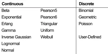
Many additional distributions can be used because of conversions made by Stat::Fit to ProcessModel distributions. See Convert Raw Data to Distributions.

Common Distributions

The following is a list of the most commonly used distributions and the syntax used to define them. The s parameter is optional (see discussion of streams following this list).

Common Distributions Syntax Components

Normal N(a, b, s) a = mean, b = standard deviation, s = stream (optional) example: N(30,5)

Triangular T(a, b, c,s) a = minimum, b=mode, c=maximum, s = stream (optional) example: T(2,10,13)

Uniform U(a, b, s) a = mean, b=half range, s = stream (optional) example: U(20,4)

User-Defined D n (% 1 ,x 1 ,…% n ,x n ) % = percentage (entries must total 100%) x = value (numeric or pre-defined descriptor) n = number of%, x entries between 2 and 5 example: D3(20, 35, 30, 45, 50, 37.5)

The following illustration shows an example of each of the common distributions:

**Triangular **This distribution is probably the most versatile yet easy to understand. It allows you to set a lower limit, an upper limit, and a most likely point. In the above example, the distribution would return a random number where the minimum value could be 2, the most likely value would be 5, and the maximum value could be 12.

For example, a call center may take as little as 1 minute with a call but usually takes 3.4 minutes and sometimes takes up to 15 minutes to complete the call. To model this in the Time field of the activity, you would enter: T(1, 3.4, 15)

Generally, you should express time values using the triangular distribution since it is flexible and realistic, yet easy to understand. Studies have shown that activity times are never uniformly distributed and rarely normally distributed. Generally, activity times approximate a triangular distribution that is skewed to the right as shown in the example above

**Normal **A normal Bell curve, this distribution allows you to designate a mean (average) and a standard deviation to generate a random number within that curve, the most likely number to be generated being the mean. The previous example shows a normal distribution with a mean or average of 30 and a standard deviation of 5.

**Uniform **This distribution allows you to generate a completely random number since any number under its curve is just as likely to be selected as any other. It is very useful when you want to have a random number unaffected by a most likely point. The previous example will result in a random number from 16 to 24 (i.e. 20 ± 4).

For example, suppose you want to assign a random number from 0 to 30 to an attribute called a_Cover_Time. Enter a_Cover_Time = U(15, 15) in the Action logic where the assignment needs to take place.

User-Defined This distribution is specialized to allow you to generate a specific number based on percentages. You can create two, three, four, or five possible outcomes. The previous example, D3(20, 35, 30, 37.5, 50, 45), will generate the number 35 exactly 20% of the time, 30% of the time the number will be 37.5, and 50% of the time 45 will be the number.

For example, two types of patients require different preparation times. About 38% of the time a nurse takes 25 minutes to prepare the patient and 62% of the time it takes 43 minutes. Enter D2(38, 25, 62, 43) in the Time field of the preparation activity.

To see the parameters for other distributions found in ProcessModel, select the Action tab for an Activity and select Distributions from the drop down filter. Select the desired distribution then select the Paste button to move a distribution into action field. This will show the parameters used to build up a distribution.

To determine what distribution to use in the absence of raw data, use the following table:

Characteristics Possible Distribution

Unboundedsymmetrical about the mean unbounded distribution skewed to the left unbounded distribution skewed to the right Normal Extreme Value IA Extreme Value IB

Bounded above a minimumTime to a random event - time between arrivals Time to a complex event - failure times Time to task completion - service times, repair times Exponential Gama Gama

Bounded between and minimum and a maximum Time to task completion- when the minimum is not more than 3 * (Max -Most likely)

• when the Maximum is not more than 3 * (Most likely - Minimum)
• Other Triangular Beta

For detailed information on all available distributions, use the Stat::Fit Help or the Stat::Fit user’s guide found in “C:Program FilesProcessModelx.xStatFitSF Manual V2.pdf”.

Streams

An optional stream number (1 - 100), shown as the S in the above tables, can be used to generate independently random numbers for the distribution. If this option is omitted, ProcessModel will use stream 1. The range is 1 - 100. The stream number is used to start the random seed value of a distribution at a number other than 1, which is the default. The stream number, preceded by a comma, is included as an additional parameter at the end of a distribution. It is placed before the closing parenthesis.

• Any negative values returned by a distribution that are used for a time expression will be automatically converted to zero.

Randomly assigning an attribute value

An entity attribute is assigned a different value or descriptor based on a random percentage. This applies to both predefined attributes such as Cost and user-defined attributes that are defined in the Attributes & Variables dialog under the Insert menu.

Suggested Technique

• Define the entity attribute.

• Assign a value or descriptor to the attribute in Action logic using the user-defined distribution function. For example: Color = D2(30, red, 70, blue)

Example: Eighty percent of the time an insurance claim form is for personal injury and 20% of the time for property damage.

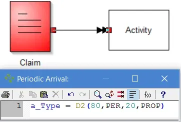
TO DO: Define the descriptive attribute called Type in the Attributes & Variables dialog under the Insert menu with PER and PROP as descriptors. Enter the Action logic as shown above in the arrival’s Action logic tab.

Related to Entity

• What is an Entity?
• What is Entity Cost?
• How do I change Activity Time based on Entity Attribute?
• How do I Change Activity Time Based on Recurring Entity Passes?
• How do I Divide an Entity?
• How do I Randomly Assign Entity Attribute Values?
• How do I Renege an Entity?
• How do I Tracking Entity Conditions?
• How do I Change Entity Graphics During Simulation?
• Why am I Getting Entity Arrival Failures at the End of Simulation?
• Why am I Getting Entity Exits System Before Releasing all Captured Resources?

Random interval arrivals

An average number of entities arrive randomly throughout a specified period. Useful in modeling situations where no specific pattern seems to exist.

Suggested Technique

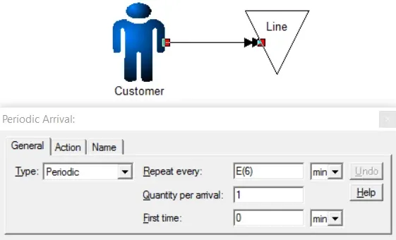
• Connect the entity to the storage or activity.
• Select the connection and choose Periodic from the Type pull-down box.
• Enter a distribution to create randomness in the Repeat every field. (The exponential distribution is recommended, e.g., E(10) would yield a random time period with an average of ten minutes.)
• Enter the number of entities to arrive during the period. (This is usually left at the default of 1 .)

Example: A car wash gets an average of ten customers per hour arriving at random intervals. (This can be reduced to one customer about every six minutes.)

TO DO: Connect the Customer entity to the Line storage (where customers wait in line) and select Periodic from the Type pull-down box. Enter a distribution of E(6) to create an arrival about every six minutes.