SimRunner

To experiment with a model’s settings and compare options, use Scenarios: define the parameters you want to vary, run the scenarios, and compare the current state against a future state side by side. The full original SimRunner guide is kept below for reference.

LegacyHow this worked in the previous version

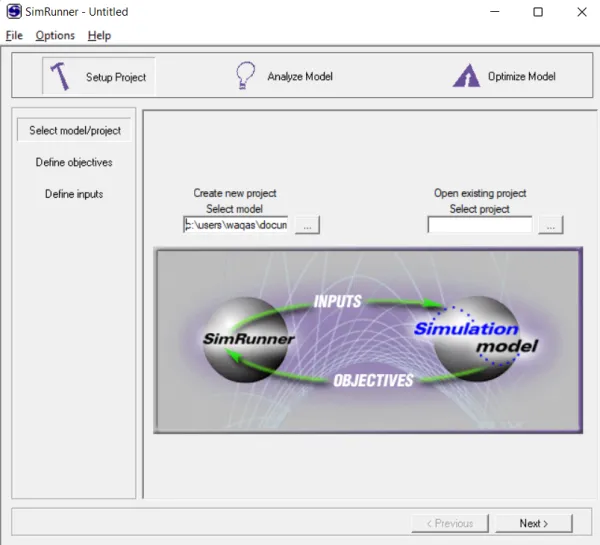
Simrunner is a tool to intelligently optimize models towards an improvement goal. For every optimization project, SimRunner employs advanced optimization algorithms to enhance multiple factors at the same time, based on a validated model, an objective function to assess system performance, and a set of factors that SimRunner can modify to enhance system performance.

SimRunner in ProcessModel

Where Do I Begin?

Start with a validated model. Once you complete and validate your simulation model, you are ready to begin an optimization project. If you are not working with a valid model, you don’t need to perform an optimization until the output from the simulation is valid.

Identify your simulation type. It is important to properly identify the simulation type, terminating or non-terminating. What does it mean to refer to a simulation as terminating or non-terminating? A terminating system stops when some key event occurs like the end of the day. When you come back the next day, you start fresh again. A non-terminating system is not necessarily a system that never stops production, rather it is a system that resumes from the point it left off. For both terminating and nonterminating simulations, you need to determine the appropriate run length and number of replications. For non-terminating simulations it is also necessary to determine the warm-up period.

Determine if the model is a true candidate for optimization. Not every simulation model is built with the express purpose of optimizing some particular element. Many simulation models are built to demonstrate the relationships that exist between various elements of your system. If optimization is appropriate, define the objective function, the output statistics used to measure the performance of proposed solutions.

Use simulation to identify and examine potential solutions. Simulation has always been trial and error when it comes to optimization. We have some sort of optimization method that we apply to the model and we examine the model’s output statistics to see if we achieved the desired outcome. This is not a bad approach if you have one decision variable you are trying to optimize, but what if you are trying to optimize multiple decision variables at once? Interaction becomes very complex and requires more advanced optimization methods like SimRunner.

Define scenario parameters. When you build your model, you must define a scenario parameter for any variable you want to optimize. This provides SimRunner with a series of values it can change as it seeks to optimize your model. In SimRunner, these values are called factors. For information on how to add and modify Scenario Parameters see Scenario Parameters.

Screen factors. Part of the simulation process is to evaluate the relationships that exist between model elements, or factors. Often, you will take the time to adjust some part of your model to find that the adjustment has no impact on system performance. Factor screening is the process of identifying which model elements (factors) do not affect the output of your model, and narrowing your search to include only those factors that affect the model’s output. Be discriminant in your selections.

Relax and wait. While some models contain relatively few factors that you can quickly optimize, others contain many. In a previous inventory reduction project, a high-end computer took approximately 24 hours to compute what it estimated to be the optimal value for the model. Although it took a long time to produce this result, the net savings were tremendous.

Consider the results. While there is no promise that SimRunner will identify the optimal solution to your process, it is possible. SimRunner will, however, find better solutions than you would likely get with your own trial and error experimentation. The surest way to know the optimal solution to any model is to run an infinite number of replications of all possible inputs. Since this is not an option, take into consideration the number of experiments you are able to perform and act accordingly.

General Procedure

The following is an overview of the process you will use to perform an optimization of your system.

Create, verify, and validate. The most important preparation you can make for an optimization project is a validated model. It is not enough to simply create a model, it will profit you nothing if the model does not reflect the real operation. Once you validate the model, you are ready to begin.
Build a project. With your model prepared for evaluation, create a new SimRunner project and identify the response statistic you wish to target. Using these response statistics, define an objective function by which to gauge system performance. SimRunner will use this objective function to measure system improvement. Next, select the input factors you will allow SimRunner to use as it determines how best to achieve system improvement. When you optimize the model, SimRunner tests each input factor to seek the combination of factors that will result in the greatest improvement of model performance.
Run experiments. Once you select the input factors and define the objective function, you can use SimRunner to automatically conduct a series of experiments on your model. SimRunner runs your model for you and tests a variety of possible combinations of values. After it completes the tests, SimRunner lists the test results in order of the most to the least successful combination of factor values.
Evaluate suggestions. The fourth step is to consider and evaluate SimRunner’s suggestions. This is crucial because SimRunner will often identify several candidate solutions to your problem and you may, for reasons not addressed in the model, prefer one solution over another. You may also wish to make additional model runs (replications) and look at confidence intervals to further evaluate SimRunner’s list of possible solutions.
Apply solution. Once you identify the solution that best fits your needs, implement the solution.

Pitfalls

If you follow the general procedure stated previously, your chances of success are very good. Typically, projects fail because the:

Model is not valid
Analysis considers insignificant factors
Analysis ignores significant factors
Objective Function is inappropriately formulated
Test results are not scrutinized

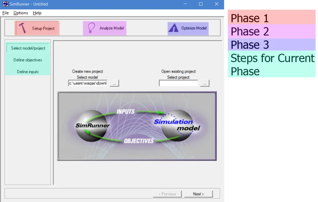
The SimRunner Interface

The SimRunner interface provides you with easy access to every step necessary to create an optimization project. The project building process is divided into three phases, each containing a series of steps necessary to complete the phase. As you move from phase to phase (displayed at the top of the dialog), a list of steps for the phase appears in the left pane.

SimRunner interface for process optimization

Set Up a Project

The first thing you must do to create an optimization project is to start a ProcessModel simulation of your model. You don’t need to complete it. The simulation just needs to be started in order to load the data required by SimRunner. After ending the simulation and returning to the modeling window, click the Tools menu and select SimRunner. The model data will be loaded automatically.

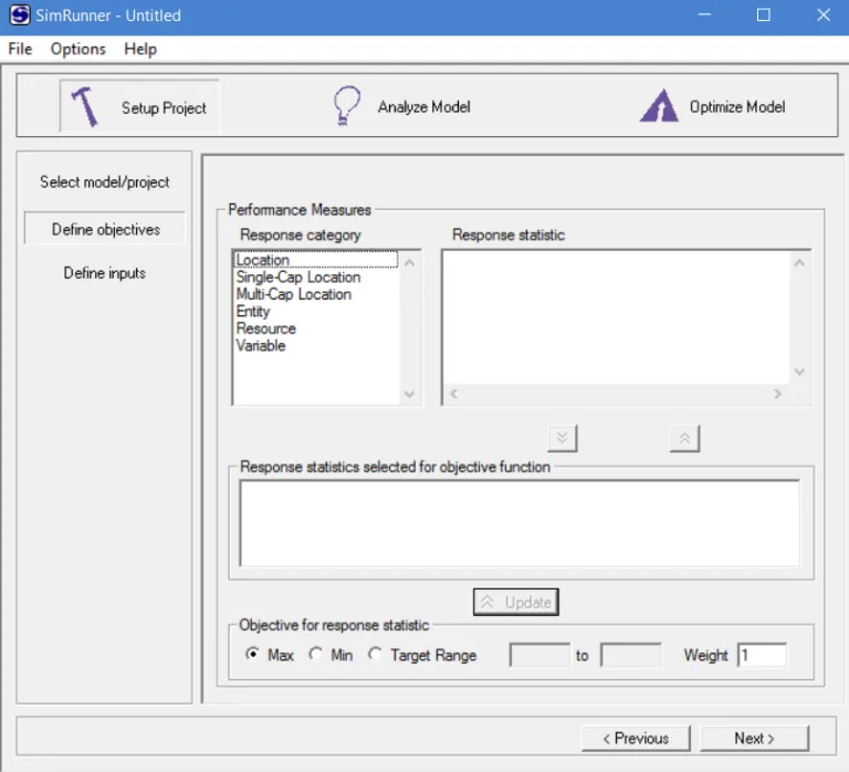
Define Objectives

The objective of your project is the final outcome you want to achieve. SimRunner measures your progress toward this goal using an objective function. An objective function is composed of response statistics, a min/max or target range, and a specific weight you wish to apply to each response statistic.

Define objectives in SimRunner

What is an Objective Function? An expression used to quantitatively evaluate a simulation model’s performance. By measuring various performance characteristics and weighting them, an objective function is a single measure of how well a system performs. SimRunner allows you to include many different performance characteristics in one objective function. For example, if you want an objective function to include a measure of total entities processed and resource utilization you could measure how well a certain simulation scenario ran by measuring Z, where: Z = (Total Processed) + (Resource Utilization).

Response Category. The response category is the type of statistic you wish to use to evaluate your model. Response categories include model elements such as locations, entities, resources, and variables.

Response Statistics. By clicking on one of the Response Categories, you will see a list of Response Statistics. Simply put, response statistics are those values you wish to improve. Once you define your targeted improvements, you are ready to define how you want them to perform, the objective for the response statistic.

Objective for Response Statistic. The objective for the response statistic refers to the way in which you want to effect change for that item. If you are trying to increase the overall output of a system, you would maximize the response statistic. Likewise, you could minimize the statistic or target a specific range within which you want the result. Finally, enter the reward or weight for each response statistic, larger numbers signify greater rewards in situations that require more than one objective.

Max: Check this option if you want to maximize the final value of this statistic.
Min: Check this option if you want to minimize the final value of this statistic. (Maximized objective functions return positive values; minimized objective functions return negative values.)
Target Range: Check this option to enter a specific target range within which you want the final result.
Statistic’s weight: Weights serve as a means of load balancing for statistics that might bias the objective function. Since most simulation models produce a variety of large and small values, it is often necessary to weight these values to ensure that the objective function does not unintentionally favor any particular statistic.

For example, suppose that a run of your model returns a throughput of .72 and an average WIP of 4.56. If you maximize throughput and minimize WIP by applying the same weight to both (W1 = W2), you will bias the objective function in favor of WIP. In this case, since you want to ensure that both statistics carry equal weight, you will apply a weight of 6.33 (W1 = 6.33) to throughput and 1.0 (W2 = 1.0) to WIP to make them of equal weight in the objective function. In situations where it is necessary to favor one statistic over another, balancing the statistics first will make it easier to control the amount of bias you apply (adapted from Harrell, Ghosh, and Bowden 2000). Typically, you will need to experiment with your model to identify the weight ratio necessary to balance statistics.

Response statistics selected for objective function. After you define the objective for the response statistic, you may click the Add button to include the statistic as part of the objective function. SimRunner combines the statistics into a linear combination and displays the updated objective function for the project.

Objective Function. The objective function is an expression used to quantitatively evaluate a simulation model’s performance. By measuring various performance characteristics and taking into consideration how you weigh them, SimRunner can measure how well your system operates. However, SimRunner knows only what you tell it via the objective function. For instance, if your objective function measures only one variable, Total_Throughput, SimRunner will attempt to optimize that variable. Since the objective function can include multiple terms, be sure to include all of the response statistics about which you are concerned.

SimRunner’s capacity to include many different response statistics in an objective function gives it tremendous capability. For example, the objective function below signifies that you wish to maximize the total ovens and cooktops processed while minimizing the total resource cost:

Z = Max:10 * (Total Ovens Processed) + Max:5 * (Total Cooktops Processed) + Min:2 * (Total Resource Cost)

SimRunner’s objective function is calculated by multiplying the result of each objective by its weighting factor, and then adding each product together. Maximized and Target Range objectives are positive and minimized objectives are negative. For example, if you maximize the number of entities processed, minimize their cost, and minimize the number of resources used, the formula would be:

(entities processed * wt) + (-cost * wt) + (-resources used * wt)

Using the following data for a single experiment: Entities processed = 100, Entity weight factor = 10, Cost = 25, Cost weight factor = 5, Resources = 8, Resource weight factor = 1. Your result would be:

objective function = (100 * 10) + (-25 * 5) + (8 * 1) = 867

Target Range. The target range in SimRunner is a means of applying bounds to the output values. SimRunner calculates the mean of the range you specify. The closer an entity is to that mean, the higher the value that element of the objective function returns. If the value returned is below the mean, the formula is Weight * (Value - Min); if above the mean, Weight * (-1) * (Value - Max); if equal to the mean, take either calculated value. The key to using the target range is that it must be a RANGE of possible values; if you defined the target range as 400 to 400, the range would be 0 and you would never get a value besides 0 out of that element.

Define Inputs

In every system, there are controllable and uncontrollable factors that determine the outcome of the process. Controllable factors include staffing, equipment, schedules, and facilities. Uncontrollable factors refer to such things as arrival rates. SimRunner allows you to target controllable model factors and determine which combination of values for those factors will elicit the behavior you desire. With each test it performs, SimRunner examines the results to see if the results will produce the effect you require from the objective function.

Defining inputs in SimRunner

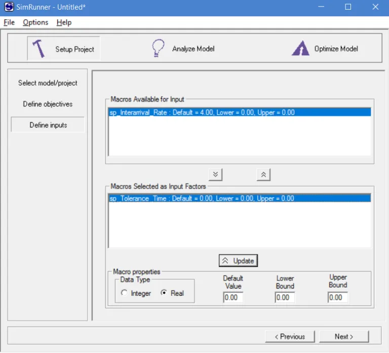
Scenario Parameters listed in model. All Scenario Parameters defined in your model are displayed in SimRunner as Macros. SimRunner will use these Scenario Parameters to improve the value of your objective function. Typically, these are the controllable factors of your model. (A scenario parameter is a placeholder for an often-used expression; you can create it once, then substitute its name anywhere in the model to use its value.)

Scenario Parameter Properties. Scenario Parameter properties describe the basic attributes of each Scenario Parameter used in your project.

Data Type: the numeric type of the data (integer or real) SimRunner will use. Typically, you will use integers to represent the number of resources (e.g. people) and real numbers to represent time values or percentages.
Default Value: SimRunner’s initial setting for the Scenario Parameter, the value SimRunner will use to analyze the model before conducting the optimization.
Lower and Upper Bound: The limits (constraints) within which this value must fall during subsequent tests.
Scenario Parameters Selected as Input Factors: A list of all Scenario Parameters you selected for use as input factors. Typically, you will want to use as few inputs as possible, only those you anticipate will affect the value of the objective function.

Define Scenario Parameters. Before you can use a model element as an input factor, you must define a Scenario Parameter for that element. To use a variable from your model as an input factor, define a corresponding Scenario Parameter and set the variable equal to it (in the variable’s “initial value” field or in the model’s processing logic). To use a resource or activity capacity as an input factor, define a Scenario Parameter that represents the capacity and place it in the appropriate field. For instance, if you have a resource named Operator_1, you can create a Scenario Parameter named Number_Of_Operators to represent the “number of units”; testing this factor will change the number of units of Operator_1 in the model. (SimRunner will not recognize a Scenario Parameter containing non-numeric characters as a valid input.)

Analyze Model

The first step in conducting any analysis of your model’s output is to make sure your model produces output with the degree of accuracy you desire. In most models, random variance is present in several places, so the output is also random. Think of a simulation experiment as a sampling technique: since you don’t know the exact population statistic, the best you can do is collect a sample large enough to make a good estimate, you must run multiple replications. SimRunner helps you select the appropriate number of replications for both terminating and nonterminating systems.

For non-terminating systems, at the very beginning of a simulation run the model is “empty” (no entities, statistics at zero). This is an artificial condition, so you must run it long enough for the operation to stabilize, to reach steady state. The warm-up time is how long it takes to reach steady state, and the end of the warm-up time is the point at which you want to begin sampling data. SimRunner uses an approach based on Welch’s graphical method: it displays a time series graph of the objective function’s current value and moving average; as the objective function stabilizes, the moving average graph appears to “flatten out” around a value, which signals the end of the warm-up period. If you are unable to determine the warm-up period from the graph, run the model again with a longer run length.

Experimental Parameters:

Simulation Run Length: The total duration of the simulation. For a non-terminating simulation, the run length should be sufficient to allow the model to warm up and reach steady state.
Output Recording Time Interval (period): SimRunner records output statistics during regular time intervals. The recording interval should be large enough to ensure that simulated events occur and the model produces an output value for each response statistic.
Number of Test Replications: The number of replications needed to conduct the analysis (five or more, depending on how long you can wait).
Percent Error in Objective Function Estimate: How accurate your estimate needs to be. Entering 10 means you wish to estimate the required replications to get the average objective function within 10% of its true value.
Confidence Level: The confidence level (90%, 95%, or 99%) used to approximate the number of replications. The higher the confidence level, the larger the number of replications needed.

Conduct Analysis / Start Analysis: Run begins analyzing the model; Final Report produces an analysis report; Analysis Status displays completion status; Warm-up handles detection for steady-state estimates; the Moving Average Window adjusts the number of periods used to compute the moving average plot. Enter the number of warm-up periods to use when estimating the required number of replications; the No. of Replications field updates automatically.

Optimization Concepts

Often, the reason for building a simulation model is to answer questions such as “What are the optimal settings to minimize (or maximize) a performance measure?” You can think of the simulation model as a black box that imitates the actual system: when you present inputs (decision variables or factors), the box produces outputs that estimate how the actual system will respond. The goal is to locate the optimal value for each factor that minimizes or maximizes the performance measure of interest.

If you were to evaluate all combinations of the different values for the input factors and plot the output response, you would create a response surface. Think of the response surface as a mountainous region with many peaks and valleys: for a maximization problem you wish to climb to the highest peak; for a minimization problem you wish to descend to the lowest valley. Once you reach a local optimum, the surest way to know it is the global optimum would be to try every possible combination, which is not feasible for most problems. What you can do is find and compare several local optimums, which greatly increases your chance of finding the global solution.

When setting up your optimization, you can do several things to greatly improve SimRunner’s performance:

Limit the number of input factors. Each factor you add increases the time necessary to optimize the model, so the fewer the factors, the faster the results.
Set good, tight bounds. It takes a lot longer to find an answer between 1 and 1000 than between 1 and 10.
Formulate a good objective function. Since SimRunner uses the objective function to evaluate a solution’s performance, include the right output responses. Your answers are only as precise as the system’s randomness allows.

SimRunner Optimization Techniques. SimRunner seeks the optimal solution by applying advanced search techniques based on Evolutionary Algorithms (Goldberg 1989, Fogel 1992, Schwefel 1981). Evolutionary Algorithms are a class of direct search techniques based on concepts from the theory of evolution: they manipulate a population of solutions so that poor solutions fade away and good solutions continually evolve in the search for the optimum. They provide not only a single, optimized solution, but many good alternatives.

Optimization Options. SimRunner provides three optimization profiles, Aggressive, Moderate, and Cautious, reflecting the number of possible solutions SimRunner will examine. The cautious profile considers the highest number of possible solutions (the largest population); aggressive considers the fewest (the smallest population). As you move from aggressive to cautious you will most often get better results, but an aggressive profile generally converges more quickly. The Convergence Percentage controls how close the best and the average solution must be to each other before the optimization stops: a high percentage stops the search early, a very small percentage runs the optimization until the points converge. Under Advanced Options you can set the Max and Min number of generations (a generation is a complete cycle of evaluating a population of parent solutions and selecting the best to produce offspring for the next generation).

Simulation Options. Disable Animation (uncheck to activate the animation during a run; enabling it takes longer but does not affect results); Number of Replications per Experiment; Warm-up Time; Run Time; and Confidence Level (if you specify more than one replication, SimRunner computes and displays a confidence interval). Typically you want SimRunner to run the algorithm until it fully converges: set a very low convergence percentage such as 0.01 and, in advanced mode, a very high maximum number of generations such as 99999 and a minimum of 1.

Seek Optimum

Seek optimum in SimRunner

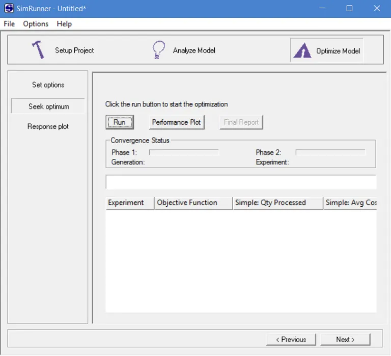
Run: Begin optimizing the model.
Stop: Halt the optimization.
Performance Plot: Plots the best objective function value found throughout the optimization process.
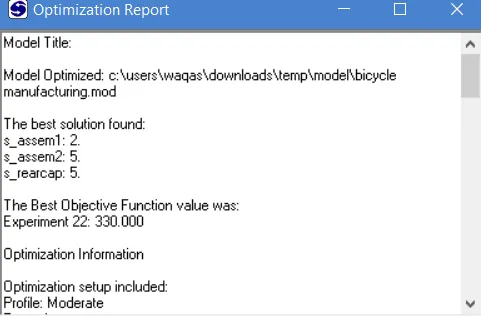
Final Report: Contains several of the best solutions found, sorted so you can evaluate them before your final decision. Results can be saved to a file using Export Optimization Data in the File menu.

Convergence Status. SimRunner sometimes uses a genetic algorithm before the evolution strategies algorithm, based on the characteristics of the problem. Phase 1 displays the convergence status of the genetic algorithm; Phase 2 displays the convergence status of the evolution strategies algorithm. Generation shows the current generation (a collection of experiments); Experiment shows the current simulation experiment.

Response Plot. Select the input factors (Independent variable 1 & 2) you wish to use to produce a partial response surface of the model’s output. Update Chart refreshes the chart; Edit Chart accesses the controls to change the appearance of the Surface Response Plot.

Optimization report in SimRunner

File Menu: New (starts a new project), Open Model, Open Project, Save, Save As, Export Optimization Data (exports the optimization grid to a comma-delimited file), Recently Opened Files, Exit.

Options Menu: Clear Optimization Data, Clear Analysis Data, Advanced (controls Minimum and Maximum Generations).

Help Menu: Help Topics, About SimRunner (shows the version).

Getting Started

In this chapter, you will create a new project from a validated model that contains Scenario Parameters and examine how the model might perform more optimally.

Simulate Model. From ProcessModel, load your model and begin a simulation (you can end it as soon as it starts). Start SimRunner by clicking the Tools menu and selecting SimRunner. The example used in this chapter is the Bicycle Manufacturing demo model available within ProcessModel. To learn by going through an example, see Case Study 5 in the Self Teaching Guide.
Define Objectives. Select the response category and statistic for each item you wish to monitor. Click Add (the down arrow button) and the statistic appears in the selected response statistics window. Enter the objective (Max, Min, Target range) and the weight, then Update. Repeat for other statistics, then click Next.
Define Inputs. Select a Scenario Parameter from the Scenario Parameters list (what are termed Scenario Parameters in ProcessModel are termed Macros in SimRunner). Click the down arrow to add it to the input factors list. Select the numeric type, then enter the default value, lower bound, and upper bound, and Update. Repeat for other parameters, then click Next.
Set Options. Select the optimization profile and enter the convergence percentage. Select the confidence level. Enable or disable the animation and specify the number of replications per experiment. Enter the warm-up time and run time. Click Next or Seek Optimum to continue.
Seek Optimum. Click Run to start the optimization. A plot of the optimization displays automatically (it can also be opened later with the Performance Plot button). View the optimization data, then click the Final Report button to display a written summary.
Response Plot. Enter the independent variables (Scenario Parameter input factors) for the response plot and click Update chart. To modify the appearance of the graph, click Edit Chart.

How SimRunner works

SimRunner uses both genetic and evolution strategies algorithms, its primary algorithm being evolution strategies, based on the work of Dr. Royce Bowden and other experts. An evolutionary algorithm is a numerical optimization technique based on simulated evolution: solutions must adapt to their environment in order to survive. Since each potential solution returns a specific result, you establish an objective function to measure the performance of each solution.

Consider this analogy. If you and a group of explorers found yourselves on the slopes of a mountain, in the dark, with nothing but radios and altimeters, how would you find the summit? First, record each person’s altimeter reading. Then direct the group to wander out in any direction for various distances and take new readings; some will have moved higher and some lower. By comparing readings you can determine the general direction in which to proceed (toward the highest reading). Repeat the process; by taking the average of the group’s readings you can confirm you are moving in the right direction. As you repeat, the group converges upon a single point. Once your average altimeter reading equals the best in the group, you have converged upon the summit. This is how SimRunner works, only the terminology is different: instead of altimeters, explorers, and tests, you use objective functions, input factors, and replications, and each time the explorers move, SimRunner calls it a generation.

Not an exhaustive search. You don’t want an algorithm that does an exhaustive search. In one inventory reduction project, modelers estimated the number of possible solutions at around 9.38 x 10^37; an exhaustive search for the optimum would take a lifetime. What you want is an algorithm that can efficiently explore the response surface and focus on the areas returning good answers, without evaluating everything.