

ProcessModel 7 Self Teach GuideChapter 3
Chapter 3. Make Your Times Vary
By the end of this chapter you can
Make work times vary, from your own data or by hand.

Before you start
In Chapter 2 every time in the shop was fixed: a customer exactly every 10 minutes, a repair exactly 12. Real work is never like that. One repair is a quick screen swap, the next a stubborn fault; customers come in clumps and gaps. This chapter teaches you to give the model times that vary, the way real times do.
Why does it matter? Because averages hide waiting. With fixed times, two Technicians kept up with no line at all. With times that vary, the same shop, with the same averages, sometimes gets two long repairs back to back while customers keep coming, and then people wait. A model with fixed times would tell you the shop is fine when it is not.
A time that varies is written as a distribution: a rule that says which times are likely and which are rare. You will set one three ways, the three you will use in real projects:
| Part | Chapter 2 | Chapter 3 |
|---|---|---|
| Repair | 12 minutes | Fitted to data: 40 repair times the shop recorded, about 12 minutes on average |
| Check In | 3 minutes | Built by hand: at least 2, mostly 3, at most 5 minutes |
| Customers | One every 10 minutes exactly | At random, 10 minutes apart on average |
| Pick Up and staff | 2 minutes, two Technicians, Capacity 2 | Unchanged |
You need your Phone Repair Shop from Chapter 2 (or the practice model below) and about thirty minutes.
Step 1. Open your shop
- Start ProcessModel. The Welcome screen lists your shop under Recent Models.
- Click Phone Repair Shop to open it.
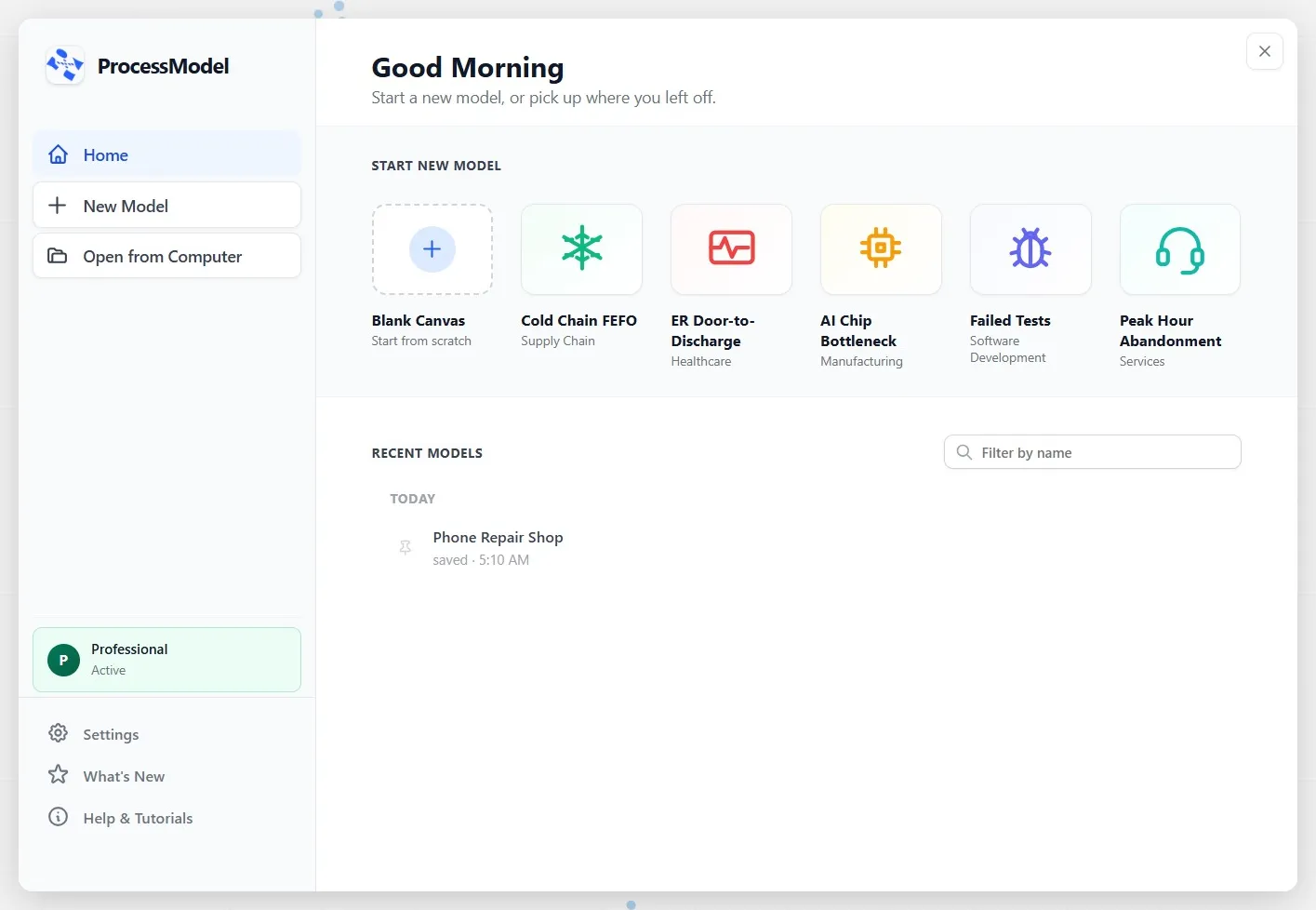
What you should see: the shop just as you left it, with two Technicians and Repair’s Capacity at 2.
Step 2. Fit Repair’s time to real data
When you have records of how long a job really took, let the data choose the distribution. That is the most honest way, because it describes your work, not a guess about it.
The shop recorded 40 repair times, in minutes. They are made up for this course, not real customer data, but they behave like real records: most repairs take about 10 to 13 minutes, a few are quick, and two run close to 25.
The 40 repair times, one per line, to copy
10.512.010.611.212.49.412.57.611.324.86.07.57.611.211.615.35.321.116.915.45.49.010.18.012.715.914.211.015.610.311.017.08.213.69.011.59.110.512.624.9- Click Repair. Its Processing Time reads 12.
- Click the button beside the Processing Time box. Time Expression opens, on its Fit Data to Distribution tab.
- Click in Sample Data and paste (or type) the 40 times, one per line. Count, under Data Summary, reads 40.
- Click Analyze.
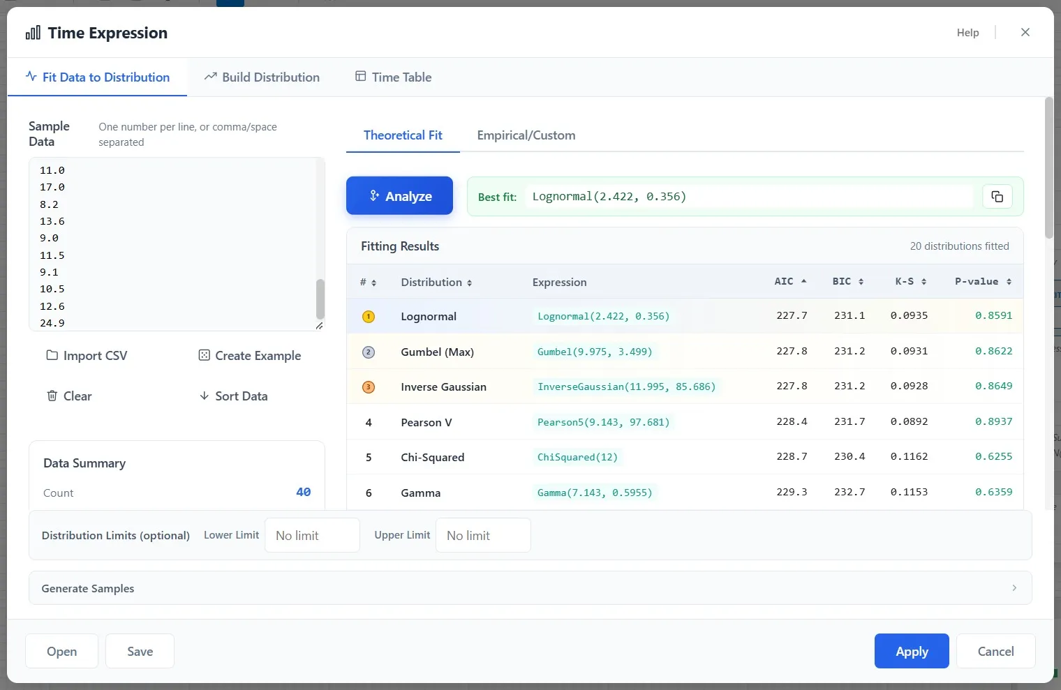
What you should see: twenty distributions fitted to your data and ranked, best first. The best, Lognormal(2.422, 0.356), is shown above the list.
Two things are worth understanding here. First, the top three (Lognormal, Gumbel and Inverse Gaussian) score almost the same, so any of them describes these repairs well; there is no need to agonize over the winner. Second, Lognormal’s two numbers are on a log scale, not in minutes, so do not read 2.422 as a time. What matters is the shape: most repairs near the middle, with a long tail of slow ones.
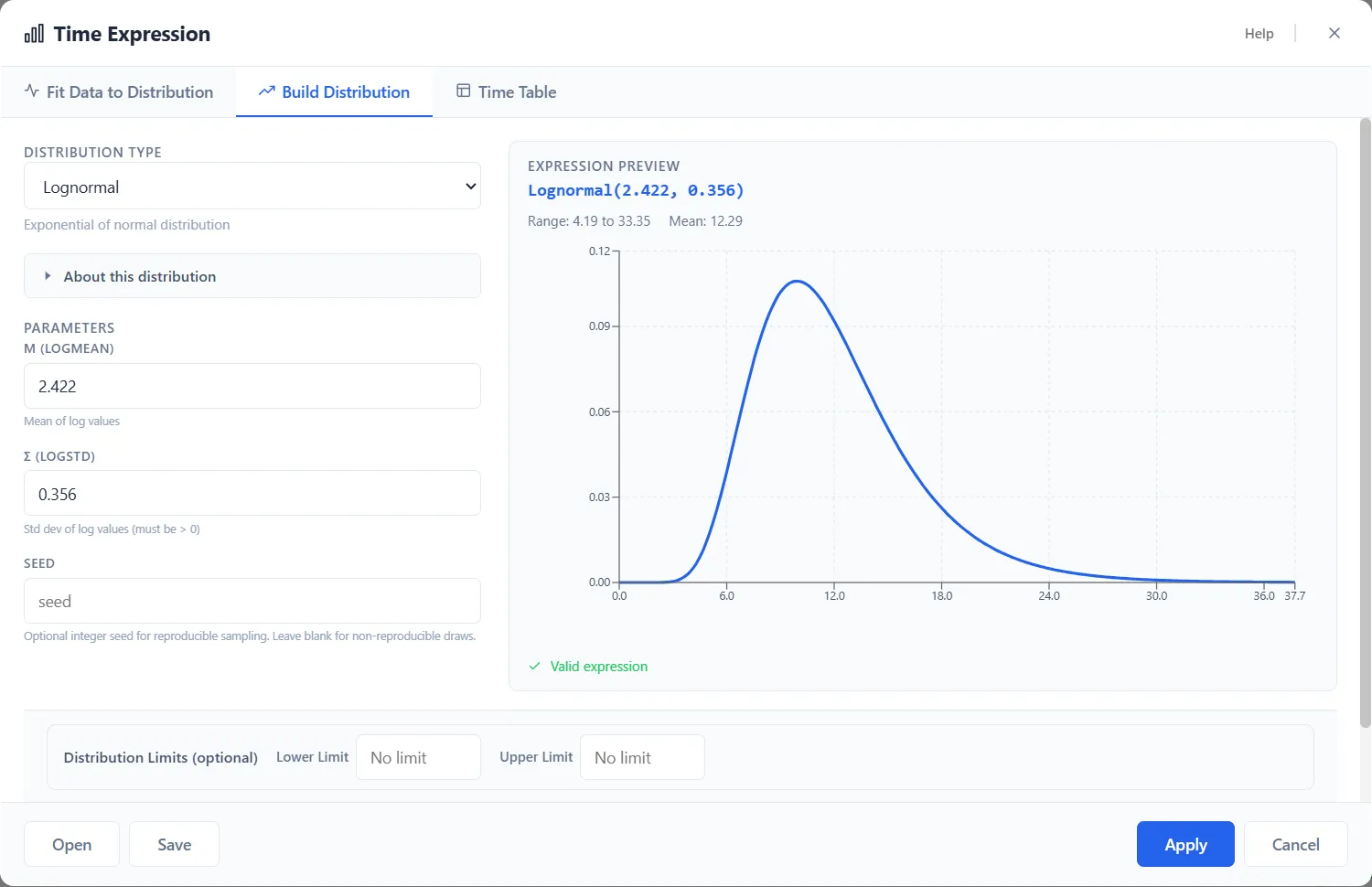
- Click Apply. A question asks whether to save the data with the model. Click No: the fitted distribution is all the model needs.
What you should see: Processing Time now reads Lognormal(2.422, 0.356), and M is still chosen. The numbers in a distribution take the unit of the field, so the times it draws are in minutes.
Step 3. Build Check In’s time by hand
Often you have no records, but the people who do the work know it well. Ask them three questions: what is the least it ever takes, what does it usually take, and what is the most? Those three answers make a triangular distribution.
For Check In, the staff say: at least 2 minutes, mostly 3, at most 5.
- Click Check In. Its Processing Time reads 3.
- Open Time Expression with the button beside the box, and click the Build Distribution tab.
- Distribution type is already Triangular, and A (min), its least value, is already 2.
- Type 3 in M (mode), the most likely time, and 5 in B (max), the most.
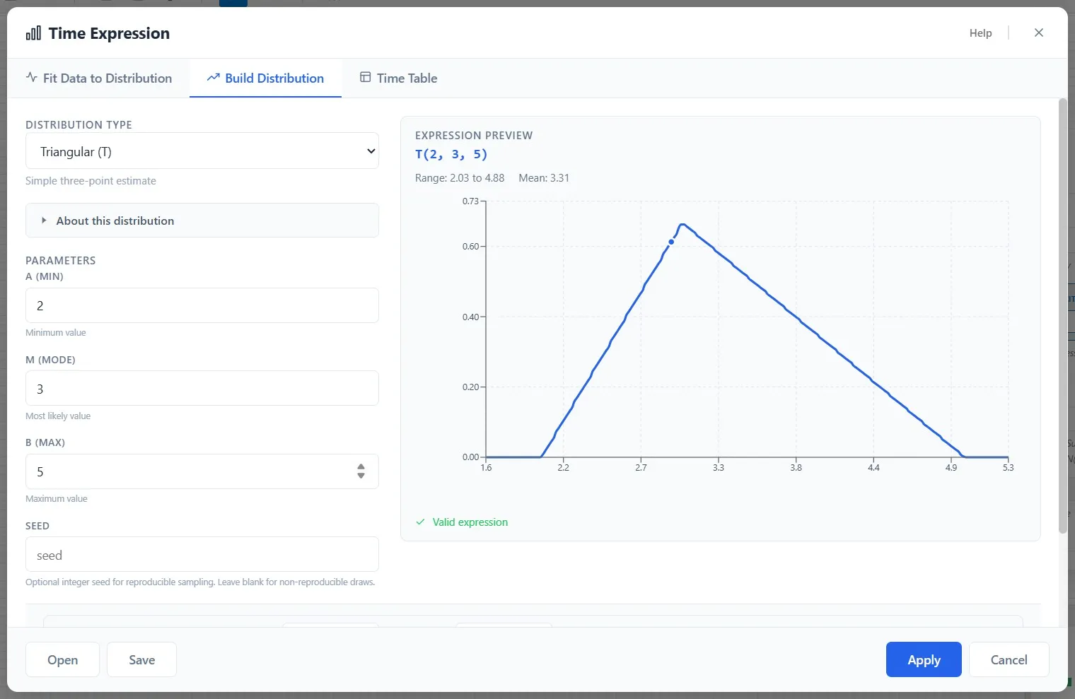
What you should see: the preview writes it as T(2, 3, 5), T for triangular, and draws its shape: most check-ins take close to 3 minutes, none less than 2 or more than 5.
- Click Apply. Processing Time now holds T(2, 3, 5), still in minutes.
Step 4. Make customers arrive at random
Customers do not walk in on a timer. They come at random: one every 10 minutes on average, but sometimes two in a minute and sometimes nobody for half an hour. Short gaps are common and long gaps rare. The exponential distribution is made for gaps like these, and it needs only one number, the average gap.
- Click the arrival line, from Customer to Check In. Time between arrivals reads 10.
- Its Time Expression button sits under the box, on the unit row. Click it, then click Build Distribution.
- In Distribution type, choose Exponential.
- Type 10 in M (mean), the average gap in minutes.
- Click Apply.
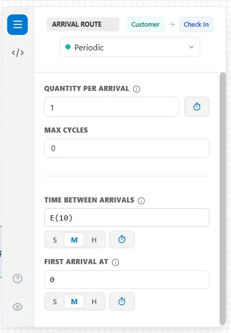
What you should see: Time between arrivals reads E(10), E for exponential, with a mean of 10, still in minutes.
Look at what you have done: you changed no average. Customers still come every 10 minutes on average, Check In still averages about 3, Repair about 12. Only the variation is new. Now see what it does.
Step 5. Run one day and watch
The run settings are the ones you set in Chapter 2: 8 hours, run once.
- Click Run Simulation.
- Watch the top left corner of Repair. When both Technicians are busy and another customer is ready, that customer waits, and the blue count shows there.
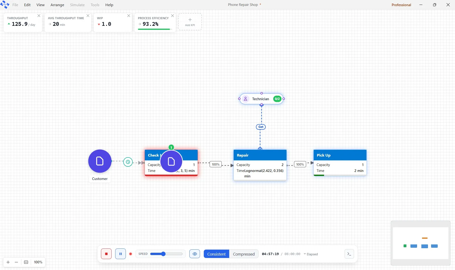
What you should see: the count on Repair’s corner comes and goes, one or two at a time, and clears again. In Chapter 2, with fixed times, it never appeared at all.
Step 6. Read the cards
When the day ends, read the cards before you answer Simulation Complete.
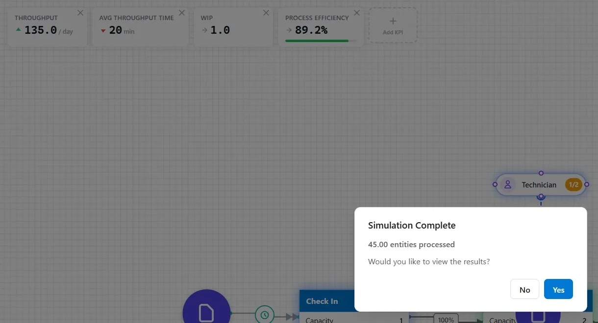
- 45 customers went through. Throughput reads 135 per day.
- Avg Throughput Time, 20 minutes, up from 17 in Chapter 2. Customers now wait at times.
- WIP, 1, where Chapter 2 ended on 2. WIP counts who is inside at this moment, so it moves all day; at the end of a run it tells you little.
- Process Efficiency, 89.2%, down from 100%. The lost share is time spent waiting.
The shop, its staff and every average are the same as in Chapter 2. Variation alone added the wait. That is why real models need real variation.
One caution: this is one run, so it is one possible day. A different day, with different random customers and repairs, would give somewhat different numbers. Chapter 10 runs many days and reads them together. Click No.
Step 7. Save it
- Click File, then Save.
What you should see: a short note that the model was saved, and the star (*) that marked unsaved changes leaves the title bar. The shop keeps its name, Phone Repair Shop. Chapter 4 starts from it.
Your practice model
- Start fromChapter 2. Your First ModelThe shop as Chapter 2 left it. Use your own saved Phone Repair Shop instead if you built it.
- Compare withChapter 3. Make Your Times VaryThe shop as this chapter leaves it. Open it when you are done, and check your settings against it.
Both are in File ▸ Demo Models, in the Self Teach Guide group. A demo model opens as a new model, so the original never changes.
Check yourself
Try it yourself
The top three fits scored almost the same. Does it matter which one you pick? Find out.
- Click Repair, open Time Expression from its Processing Time, and paste the 40 times into Sample Data again. Click Analyze.
- Click the second row, Gumbel (Max), to choose it instead of the best fit, and click Apply (answer No to saving the data).
- Run the day again and read the cards before you answer Simulation Complete.
Mark it done
When you can say which of the three ways to set a time you would use, and why, turn on Done.
You watched this chapter's video.Not watched yet: the video is marked when it plays to the end.
Kept in this browser only, and shown on the course page.