
In an Oregon hospital, a modeler learned a technique to build accurate models in two days. Not models of a single interaction, but models of an entire department, such as surgery or maternity, or the overall flow of the hospital. In this article you will learn three concepts that speed up modeling, and you will see how to be fully confident in both the model and its results.
Article summary
The usual way to develop a simulation model takes considerable time to analyze data, verify operation, and validate the statistical characteristics of the model.
This article shows an alternate technique called Real Data Modeling. It uses actual product or patient records to drive the model, where each record carries its own routing, duration, resource requirements, and so on. The data is pulled from company systems and read into ProcessModel.
It sounds difficult, but it is not. A real data model can be built in a fraction of the usual modeling time, and testing is simple because known inputs produce known outputs. You can feed in a past production schedule and check the result against the production reports you already have. Faster modeling means quicker decisions, and quicker decisions mean improvements on the things management still cares about.
Get to the decision
The most common reason to build a model is to answer a question, and to answer it with certainty. We model because the entire interaction can be captured and understood, and because we want to be sure.
Statistical models are built by analyzing past data to predict what could happen in the future. Every statistical model has to go through a rigorous, time-consuming process to verify it before anyone can trust the output.
An alternate approach
The alternative is to use actual data from a previous period to drive the model. For a surgical suite, a real patient record supplies the date, the time in preop, the suite needed, the surgical time, the post-op time, and so on. For a manufacturing facility, actual orders supply quantity, routing, setup time, batch size, and work time. No distributions are needed for this technique.

Some of the advantages of Real Data Modeling:
- Very fast model builds
- Simple, quick validation, because you compare actual inputs against known outputs
- Very high model accuracy
- Change the model by changing the input
What is the theory?
Keep it simple. When you use actual times and requirements, you can see the performance that proposed changes would make possible. If a change would have made a difference last year, then it can be projected onto this year. For example, you can stop the simulation when the production orders complete and record the hours required. After making a change, run the model again, compare the new hours against the recorded hours, and calculate the improvement. Keep it simple.
An Indiana manufacturing company produces 170 different products on a single production line, each with unique routings and workstation times. The routings, setups, and station times come from the company database and are read in through a spreadsheet. Historical records give the past production schedules, which are read in the same way. Within days, the company was answering questions such as:
- Which products should be close together in the production sequence?
- Which products should be far apart in the production sequence?
- What were the optimal batch sizes?
- Which products should move to another line?
- What will increase production?
- Where are the best investments to increase production?
The model became a fast way to run a kaizen study. Ideas became experiments and were tested within minutes. As a result, the company improved production by more than 40%, and the project cost was low.
How to build a Real Data model
There are three main steps to a Real Data model.
- Build the model to handle any order of routing.
- Build the logic to extract the routing information from entity attributes.
- Prepare the arrivals to carry the attribute information.
Build the model to handle any order of routing
Think of the model as generic, built to handle any routing order. Send every entity to a common location where it picks up the information it needs to route to its first activity, along with how much processing time that activity will take. When it finishes at the first activity, it returns to the common location and picks up the information for the second location and its processing time, and so on.
In this structure, all entities enter the common location. Conditional routes read a common attribute to steer each entity to the next location, and once it arrives, the processing time comes from another common attribute. When the entity finishes, it routes back to the common activity to pick up the next location and time. A simplified healthcare example illustrates the idea.
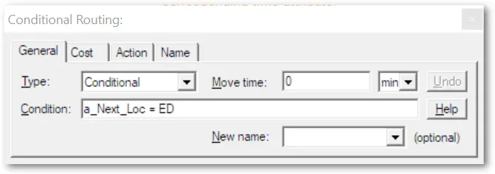
Routes drawn in blue are percentage routings. The black box is a dummy activity that consolidates all the blue routes from the locations so that a single route goes back to the director. Routes drawn in red are conditional routings. Here is an example conditional route into the ED:
In a healthcare environment, the number of locations might grow to 20, but the technique works in any industry, and the base model could be expanded to hundreds of locations if needed. To adapt the model to your own locations, you change the activity names, change the conditions in the conditional routes, and change the logic described below.
Build the logic to extract information from entity attributes
All of the model’s logic lives in the director activity, and it is simple. Each time an entity enters the director, its counter attribute is incremented. The first time through, the location is read from the first location attribute and the processing time from the first time attribute. The second time through, the location and time are read from the second set of attributes, and so on:
INC a_Loc_CountIF a_Loc_Count = 1 THEN ...ELSE IF a_Loc_Count = 2 THEN ...ELSE IF a_Loc_Count = 3 THEN { a_Next_Loc = a_Loc3 ...etc.The attribute a_Next_Loc is used in every red conditional route to steer the entity to its next location, and a_Next_Time is used at every location to set the processing time. Every location uses the same attribute for processing time, as shown in this dialog:
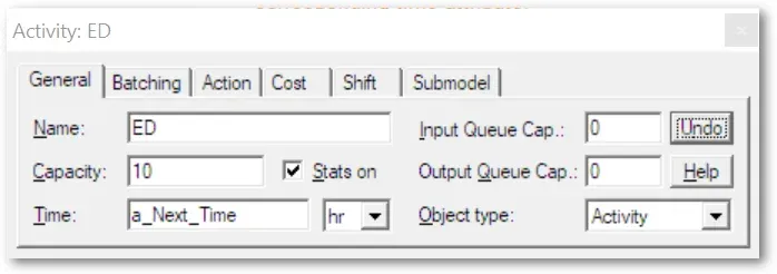
Additional attributes are added to account for other aspects of the system, such as setup time or batch size.
Prepare the arrivals to carry routing information
The last step is to structure the scheduled arrival input sheet. A matching input sheet lives in the arrivals category of model objects. Example data populates the sheet:
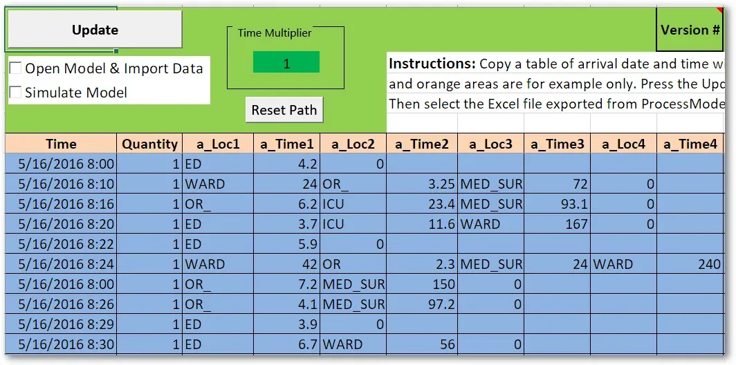
Prepare the input so that the first location goes into the attribute a_Loc1 and its associated time goes into a_Time1. The good news is that a company database usually already holds everything you need. If you want help converting your data into this format, contact support, because we have done it many times.
Show the entity how to exit
How does an entity know it has finished its routing? It returns to the director, which sets a_Next_Loc to the next value. When that attribute equals zero, the entity leaves the simulation:
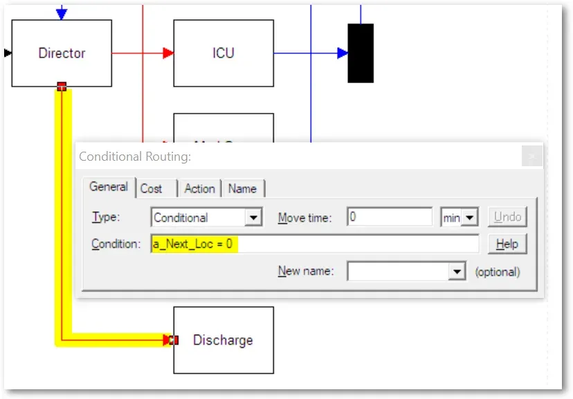
The logic in this example can be expanded to handle as many locations as you need. Real Data Modeling lets you build and experiment with models in a fraction of the time normally required, and faster modeling and analysis mean quicker decisions and faster improvements. If you are still building up your modeling foundation, the step-by-step guide to building models pairs well with this approach. To put it to work, explore what ProcessModel can do.